------------------------------------------------------------------------
BIOWULF'S MATHEMATICAL TOOLS:
-----------------------------
NEW BREAKTHROUGHS IN MACHINE LEARNING
-------------------------------------
screenplay by
Alan B. Scrivener
19 July 2001
second draft
------------------------------------------------------------------------
S-___. TITLE CARD
BIOWULF LOGO
 S-___. TITLE CARD
YELLOW LETTERS ON WATERFALL BACKGROUND:
BIOwulf's Mathematical Tools:
New Breakthroughs in Machine Learning
NARRATOR
BIOwulf's mathematical tools: new breakthroughs in
machine learning
S-___. MEDIUM SHOT: NARRATOR IN FRONT OF NEUTRAL BACKGROUND
NARRATOR (CONTINUING)
Hi, I'm Mollie Tobin, and in the next thirty minutes I want to
briefly explain some of the mathematical tools used by BIOwulf for
machine learning, especially the technique known as
"Support Vector Machines," or "SVM" for short.
This is a rather obscure phrase, becasue it's hard to
understand the meaning without a lot of explanation.
To illustrate this, we asked a 7 year old child to draw
what she imagined when she heard the words, "Support
Vector Machine." We did have to explain that a vector
is sort of like an arrow.
S-___. CLOSE UP: NARRATOR HOLDING DRAWING
NARRATOR (CONTINUING)
Here you can see there is a machine, held up by this
support, which shoots arrows.
S-___. MEDIUM SHOT: NARRATOR IN FRONT OF NEUTRAL BACKGROUND
NARRATOR (CONTINUING)
So first we may have to wipe away some miconceptions before
we present some replacement concepts. We'll get to that
in a minte. First let me tell you what we've assumed about
you.
We're assuming that you know the concepts of algebra;
maybe you took calculus in college and then forgot it all,
but you can still look at an equation like this...
S-003. CARD
YELLOW LETTERS ON BLUE BACKGROUND:
a x2 + b x + c = 0
NARRATOR (CONTINUING)
... and you realize that x is the variable and a, b and c
are constants. You remember that x superscript 2 means x
squared, or x time x, and you remember that b right next to
x there means b times x.
S-004. CLOSE-UP: NARRATOR IN FRONT OF NEUTRAL BACKGROUND
NARRATOR (CONTINUING)
Extra credit if you recognize it as "the quadratic equation."
I'd also like to apologize in advance to those of you who are
mathematicians, quantitative scientists or engineers -- for you
this information may seem overly basic, at least at first.
We want to make sure we bring everyone along. But hang
in there and I bet you'll learn something yet!
And just so you are clear on the scope of this video, this is
not to inform you of BIOwulf's business plans, key people,
product offerings or marketing message. That information
is communicated in other ways. This video will cover the
following topics...
S-005. CARD:
YELLOW LETTERS ON BLUE BACKGROUND:
Why this is important.
machine learning
generalization
overfitting
state space
combinatorial explosion
correlation
orthogonal
linear
weights
recursion
recursive feature elimination
support vectors
kernels
Does it work?
NARRATOR (CONTINUING)
First we'll get a quick reminder why this stuff is
important, and then we'll review the he concepts of:
machine learning,
generalization,
overfitting,
a state space,
a combinatorial explosion,
what is correlation,
what does orthogonal mean,
linear functions,
weights,
recursion,
recursive feature elimination,
support vectors, and
kernels,
followed by a brief discussion of perhaps the most important
question: "Does it work?"
S-006. MEDIUM SHOT: NARRATOR IN FRONT OF NEUTRAL BACKGROUND
NARRATOR (CONTINUING)
Now we're not going to explain how you can use these mathematical
tools yourself -- we have some papers you should read if you want
to get into that level. We're just going to explain in broad
outlines how they work. This quote from Richard Feynman's
brilliant little book on quantum electrodynamics...
(HOLDS UP 'QED')
-- QED is the title -- explains well what we are trying
to do:
(READING FROM THE BOOK)
"How am I going to explain to you things I don't explain to
my students until they are third year graduate students?
Let me explain it by analogy. The Maya Indians were very
interested in the rising and setting of Venus as a morning
star and as an evening star -- they were very interested
in when it would appear. After some years of observation
they noted that five cycles of Venus were very nearly equal
to eight of their years of 365 days. To make calculations,
the Maya had invented a system of bars and dots to represent
their numbers -- including zero -- and had rules by which to
calculate and predict not only the risings and settings of
Venus, but of other celestial phenomena, such as Lunar
eclipses.
"In those days, only a few Maya priests could do such elaborate
calculations. Now, suppose we were to ask one of them how to
do just one step in the predicting when Venus will next rise
as a morning star -- subtract two numbers. How would the
priest explain what subtraction is?
"He could either teach us the numbers represented by the bars
and dots and the rules for subtracting them, or he could
tell us what he was really doing: 'Suppose we want to
subtract 236 from 584. First count out 584 beans and put
them in a pot. The take out 236 beans and put them to one
side. Finally, count the beans left in the pot. That number
is the result of subtracting 236 from 584.'
"You might say, 'What tedium -- counting beans, putting
them in, taking them out -- what a job!'
"To which the priest would reply, 'That's why we have the
rules for the bars and dots. The rules are tricky, but
they are a much more efficient way of getting the answer
than by counting beans. The important thing is, it makes
no difference as far as the answer is concerned: we
can predict the appearance of Venus by counting beans (which
is slow, but easy to understand) or by using tricky rules
(which is much faster, but you must spend years in school
to learn them).'"
(LOWERS BOOK)
Got it? Okay, let's get started.
S-007. CARD: YELLOW LETTERS ON BLUE BACKGROUND:
Why this is important.
S-___. MEDIUM SHOT: NARRATOR IN FRONT OF NEUTRAL BACKGROUND
NARRATOR
I don't mean to be melodramamtic, but what we're trying to do
here is cure cancer, among other things. The point of all
this esoteric math is to improve medical diagnosis.
S-___. LONG SHOT: NARRATOR AT MISSION
NARRATOR (CONTINUING)
I'm here at Mission San Juan Capistrano, you know,
where the swallows return every year.
S-___. MEDIUM SHOT: NARRATOR IN ALCOVE
NARRATOR (CONTINUING)
This little alcove is all that's left of the oldest building
in California; today it is used as the shrine to Saint Peregrine,
the Patron Saint of Cancer Suffers.
S-___. CLOSE UP: CANDLES BURNING
NARRATOR (CONTINUING)
Over half a million people die of cancer every year.
S-___. lONG SHOT: PEOPLE AT SPORTS STADIUM
NARRATOR
That's almost ten times the number of people this stadium holds.
S-___. MEDIUM SHOT: NARRATOR IN FRONT OF NEUTRAL BACKGROUND
NARRATOR
Did you know the state of Georgia has an initiative to cure
cancer? Thye'd like to go down in history as the state it
happened in. Some thing to be proud of, to tell the grand kids.
S-___. CARD: FIGURE F-_
S-___. TITLE CARD
YELLOW LETTERS ON WATERFALL BACKGROUND:
BIOwulf's Mathematical Tools:
New Breakthroughs in Machine Learning
NARRATOR
BIOwulf's mathematical tools: new breakthroughs in
machine learning
S-___. MEDIUM SHOT: NARRATOR IN FRONT OF NEUTRAL BACKGROUND
NARRATOR (CONTINUING)
Hi, I'm Mollie Tobin, and in the next thirty minutes I want to
briefly explain some of the mathematical tools used by BIOwulf for
machine learning, especially the technique known as
"Support Vector Machines," or "SVM" for short.
This is a rather obscure phrase, becasue it's hard to
understand the meaning without a lot of explanation.
To illustrate this, we asked a 7 year old child to draw
what she imagined when she heard the words, "Support
Vector Machine." We did have to explain that a vector
is sort of like an arrow.
S-___. CLOSE UP: NARRATOR HOLDING DRAWING
NARRATOR (CONTINUING)
Here you can see there is a machine, held up by this
support, which shoots arrows.
S-___. MEDIUM SHOT: NARRATOR IN FRONT OF NEUTRAL BACKGROUND
NARRATOR (CONTINUING)
So first we may have to wipe away some miconceptions before
we present some replacement concepts. We'll get to that
in a minte. First let me tell you what we've assumed about
you.
We're assuming that you know the concepts of algebra;
maybe you took calculus in college and then forgot it all,
but you can still look at an equation like this...
S-003. CARD
YELLOW LETTERS ON BLUE BACKGROUND:
a x2 + b x + c = 0
NARRATOR (CONTINUING)
... and you realize that x is the variable and a, b and c
are constants. You remember that x superscript 2 means x
squared, or x time x, and you remember that b right next to
x there means b times x.
S-004. CLOSE-UP: NARRATOR IN FRONT OF NEUTRAL BACKGROUND
NARRATOR (CONTINUING)
Extra credit if you recognize it as "the quadratic equation."
I'd also like to apologize in advance to those of you who are
mathematicians, quantitative scientists or engineers -- for you
this information may seem overly basic, at least at first.
We want to make sure we bring everyone along. But hang
in there and I bet you'll learn something yet!
And just so you are clear on the scope of this video, this is
not to inform you of BIOwulf's business plans, key people,
product offerings or marketing message. That information
is communicated in other ways. This video will cover the
following topics...
S-005. CARD:
YELLOW LETTERS ON BLUE BACKGROUND:
Why this is important.
machine learning
generalization
overfitting
state space
combinatorial explosion
correlation
orthogonal
linear
weights
recursion
recursive feature elimination
support vectors
kernels
Does it work?
NARRATOR (CONTINUING)
First we'll get a quick reminder why this stuff is
important, and then we'll review the he concepts of:
machine learning,
generalization,
overfitting,
a state space,
a combinatorial explosion,
what is correlation,
what does orthogonal mean,
linear functions,
weights,
recursion,
recursive feature elimination,
support vectors, and
kernels,
followed by a brief discussion of perhaps the most important
question: "Does it work?"
S-006. MEDIUM SHOT: NARRATOR IN FRONT OF NEUTRAL BACKGROUND
NARRATOR (CONTINUING)
Now we're not going to explain how you can use these mathematical
tools yourself -- we have some papers you should read if you want
to get into that level. We're just going to explain in broad
outlines how they work. This quote from Richard Feynman's
brilliant little book on quantum electrodynamics...
(HOLDS UP 'QED')
-- QED is the title -- explains well what we are trying
to do:
(READING FROM THE BOOK)
"How am I going to explain to you things I don't explain to
my students until they are third year graduate students?
Let me explain it by analogy. The Maya Indians were very
interested in the rising and setting of Venus as a morning
star and as an evening star -- they were very interested
in when it would appear. After some years of observation
they noted that five cycles of Venus were very nearly equal
to eight of their years of 365 days. To make calculations,
the Maya had invented a system of bars and dots to represent
their numbers -- including zero -- and had rules by which to
calculate and predict not only the risings and settings of
Venus, but of other celestial phenomena, such as Lunar
eclipses.
"In those days, only a few Maya priests could do such elaborate
calculations. Now, suppose we were to ask one of them how to
do just one step in the predicting when Venus will next rise
as a morning star -- subtract two numbers. How would the
priest explain what subtraction is?
"He could either teach us the numbers represented by the bars
and dots and the rules for subtracting them, or he could
tell us what he was really doing: 'Suppose we want to
subtract 236 from 584. First count out 584 beans and put
them in a pot. The take out 236 beans and put them to one
side. Finally, count the beans left in the pot. That number
is the result of subtracting 236 from 584.'
"You might say, 'What tedium -- counting beans, putting
them in, taking them out -- what a job!'
"To which the priest would reply, 'That's why we have the
rules for the bars and dots. The rules are tricky, but
they are a much more efficient way of getting the answer
than by counting beans. The important thing is, it makes
no difference as far as the answer is concerned: we
can predict the appearance of Venus by counting beans (which
is slow, but easy to understand) or by using tricky rules
(which is much faster, but you must spend years in school
to learn them).'"
(LOWERS BOOK)
Got it? Okay, let's get started.
S-007. CARD: YELLOW LETTERS ON BLUE BACKGROUND:
Why this is important.
S-___. MEDIUM SHOT: NARRATOR IN FRONT OF NEUTRAL BACKGROUND
NARRATOR
I don't mean to be melodramamtic, but what we're trying to do
here is cure cancer, among other things. The point of all
this esoteric math is to improve medical diagnosis.
S-___. LONG SHOT: NARRATOR AT MISSION
NARRATOR (CONTINUING)
I'm here at Mission San Juan Capistrano, you know,
where the swallows return every year.
S-___. MEDIUM SHOT: NARRATOR IN ALCOVE
NARRATOR (CONTINUING)
This little alcove is all that's left of the oldest building
in California; today it is used as the shrine to Saint Peregrine,
the Patron Saint of Cancer Suffers.
S-___. CLOSE UP: CANDLES BURNING
NARRATOR (CONTINUING)
Over half a million people die of cancer every year.
S-___. lONG SHOT: PEOPLE AT SPORTS STADIUM
NARRATOR
That's almost ten times the number of people this stadium holds.
S-___. MEDIUM SHOT: NARRATOR IN FRONT OF NEUTRAL BACKGROUND
NARRATOR
Did you know the state of Georgia has an initiative to cure
cancer? Thye'd like to go down in history as the state it
happened in. Some thing to be proud of, to tell the grand kids.
S-___. CARD: FIGURE F-_
 NARRATOR (CONTINUING)
Biowulf is working with the state of Georgia's Department
of Community Health, which gives them access to cancer diagnosis
data for over 2 million people, in order to improve cancer diagnosis.
That's why this is important.
Okay, let's get to our first concept.
S-___. CARD: YELLOW LETTERS ON BLUE BACKGROUND:
machine learning
S-___. MEDIUM SHOT: NARRATOR IN FRONT OF NEUTRAL BACKGROUND
NARRATOR
I want to make sure you aren't confused by the word 'machine'
here. What we mean is a algorithm, or precise technique,
for solving a problem. The mathematical literature is full
of abstract machines, like the Markhov Machine and the Turing
Machine, which are just mathematical models. There usually
isn't a special physical machine built, it's just simulated
by programming a digital computer. In the case of machine
learning, we're talking about writing a computer program
that can learn rules by studying example data.
Lets really spell this out, because this is the problem
definition. I'm going to give you two made-up examples, just
because they're easy to talk about, and then a third example
that is the kind of work BIOwulf actually does with machine
learning.
First, imagine that you've discovered some unusual kind of
rat nobody knows anything about, and you want to know what
to feed it. Fortunately you have some recent dietary
experiment results for these rats. Some students had a bunch
of rats and for each one they randomly chose a particular
canned food from a grocery store and fed it only that food
daily for a month.
(HOLDS UP A CAN WITH NUTRITIONAL CONTENT LABEL)
They added up the nutritional contents
on the sides of the cans...
S-___. CLOSE UP: NUTRITIONAL LABEL
NARRATOR (CONTINUING)
...you know, the amount of vitamins, minerals, proteins,
fat and so on...
S-___. CARD: TABLE T-1
NARRATOR (CONTINUING)
Biowulf is working with the state of Georgia's Department
of Community Health, which gives them access to cancer diagnosis
data for over 2 million people, in order to improve cancer diagnosis.
That's why this is important.
Okay, let's get to our first concept.
S-___. CARD: YELLOW LETTERS ON BLUE BACKGROUND:
machine learning
S-___. MEDIUM SHOT: NARRATOR IN FRONT OF NEUTRAL BACKGROUND
NARRATOR
I want to make sure you aren't confused by the word 'machine'
here. What we mean is a algorithm, or precise technique,
for solving a problem. The mathematical literature is full
of abstract machines, like the Markhov Machine and the Turing
Machine, which are just mathematical models. There usually
isn't a special physical machine built, it's just simulated
by programming a digital computer. In the case of machine
learning, we're talking about writing a computer program
that can learn rules by studying example data.
Lets really spell this out, because this is the problem
definition. I'm going to give you two made-up examples, just
because they're easy to talk about, and then a third example
that is the kind of work BIOwulf actually does with machine
learning.
First, imagine that you've discovered some unusual kind of
rat nobody knows anything about, and you want to know what
to feed it. Fortunately you have some recent dietary
experiment results for these rats. Some students had a bunch
of rats and for each one they randomly chose a particular
canned food from a grocery store and fed it only that food
daily for a month.
(HOLDS UP A CAN WITH NUTRITIONAL CONTENT LABEL)
They added up the nutritional contents
on the sides of the cans...
S-___. CLOSE UP: NUTRITIONAL LABEL
NARRATOR (CONTINUING)
...you know, the amount of vitamins, minerals, proteins,
fat and so on...
S-___. CARD: TABLE T-1
| rat # | Carb. | Fat | Cholest. | Sodium | Protein | Vitamin A | Vitamin C | Calcium | Iron | +/- |
|---|
| rat #1 | 0 g | 0.5 g | 30 mg | 200 mg | 13 g | 0% | 0% | 0% | 2% | - |
| rat #2 | 20 g | 0 g | 0 mg | 10 mg | 1 g | 0% | 20% | 0% | 2% | - |
| rat #3 | 25 g | 2 g | 0 mg | 45 mg | 0 g | 0% | 0% | 0% | 2% | - |
| rat #4 | 4 g | 0 g | 0 mg | 0 mg | 1 g | 4% | 8% | 2% | 4% | + |
% = per cent daily human requirements
         NARRATOR (CONTINUING)
      .. and for each rat, they made a list of all of the nutrients
      it received, and a notation as to whether it lived or died.
      You can see on the list here, each row is a rat.  The leftmost
      column gives the rat number, the columns in the middle are the
      nutrients, and the last column is a plus if the rat lived and
      a minus if it died.

S-___. MEDIUM SHOT: NARRATOR IN FRONT OF NEUTRAL BACKGROUND

         NARRATOR
      The challenge then is to figure out from the list -- and only
      from the list -- what is the best diet to feed the rats.
      And to be able to take a proposed diet and predict whether
      a rat will live or die on it.

S-___. MEDIUM SHOT: NARRATOR IN FRONT OF NEUTRAL BACKGROUND

         NARRATOR (CONTINUING)
      We want to produce the formula automatically from the numbers
      in the list.  In other words, we need a program that gets
      trained by the data and then can classify new data.

      The second example is not made up, but represents actual
      research done by BIOwulf's mathematicians.

      We were fortunate to receive 62 frozen tissue samples from
      ____ hospital that were biopsies of patients with suspected
      colon cancer.  Along with the samples was a file on each
      patient covering 30 years of follow-up testing, so that it
      was possible for each sample to know the "right answer" in
      advance -- whether the patient got colon cancer or not.

      With modern genetic analysis techniques we were able to
      subject each sample to 2000 gene probes, to determine for
      each of 2000 genes whether that gene was silent, active or
      hyperactive in the sample.  In each case this was turned
      into a number from zero to one.

S-___. CARD: TABLE T-3
| patient # | income | gene #1 | gene #2 | gene #3 | gene #4 | *** | +/- |
|---|
| patient #1 | 0.56 | 0.45 | 0.55 | 0.21 | 0.98 | *** | - |
| patient #2 | 0.66 | 0.89 | 0.47 | 0.82 | 0.38 | *** | + |
| patient #3 | 0.01 | 0.09 | 0.66 | 0.63 | 0.54 | *** | + |
NARRATOR (CONTINUING)
You can see that for each patient we have a row of data on
which genes were expressed, and by how much, and in the rightmost
column a plus sign if the patient got colon cancer and a minus
if they didn't.
S-___. MEDIUM SHOT: NARRATOR IN FRONT OF NEUTRAL BACKGROUND
NARRATOR (CONTINUING)
Once again the goal is to produce a formula -- what we
call the Decision Function -- to sort patients correctly
into those who will and won't get the cancer, using only
the information on the list.
Okay, a third example: this one is also made up, but it's
designed to help you visualize what's going on more
easily.
This one is really simple. There's only two columns in the chart.
In fact, I'm not even going to show you a chart for this one.
You're sick of charts anyway, right?
Imagine there's this landscape someplace that youy can't see.
Some mountains, valleys, water, and you're trying to avoid the
water, but you have no idea what the shape of the terrain is.
So you drop probes. Each probe tells you its latitude and
longitude. If we assume the earth is flat that's just 2
dimensional grid coordinates. And we also find out if the
probe got wet or not. We get -- guess what? -- a plus if
it's dry and a minus if it's wet.
S-___. CARD: FIGURE F-__
 NARRATOR (CONTINUING)
So we draw a map of these plusses and minuses.
Essentially we're trying to guess the terrain from the pluses
and minuses.
S-___. MEDIUM SHOT: NARRATOR IN FRONT OF NEUTRAL BACKGROUND
NARRATOR (CONTINUING)
Let's dig into this metaphor a little more, and take a field
trip.
S-___. LONG SHOT: MISSION TRAILS SIGN
NARRATOR (CONTINUING)
We're here at a canyon in San Diego called Misssion Gorge.
S-___. MEDIUM SHOT: NARRATOR BEFORE GRANITE MOUNTAINS
NARRATOR (CONTINUING)
All around me you can see the striking granite geography.
Some of those same mission swallows nest in these walls, by the way.
S-___. MEDIUM SHOT: NARRATOR AT STREAM SIDE
NARRATOR (CONTINUING)
And isn't this a magical spot, down by the river?
Father Serra, founder of the California Missions, surely
walked along these banks, and before that Kumayaay natives
used grinding holes here to gring acorn flour.
But I'm letting myself get distracted.
Here we can observe water flowing, seeking its own level.
To make this metaphor work, we'll have to assume that water flows
extremely fast, seeking its own level instantly.
S-___. CLOSE UP: NARRATOR DIPPING HANDS IN STREAM
NARRATOR (CONTINUING)
So we wouldn't see waterfalls like this. All this water would
already be out to sea. Imagine if the oceans rose, though, and
filled this canyon. No surf, no waves, just a calm sea
intersecting the canyon walls.
Remember our goal, to determine for any arbitrary point whether
it is wet or dry.
Of course, the perfect solution would be if we knew the actual
elevation at each point.
S-___. CLOSE UP OF TOPO LINES ON MAP
NARRATOR (CONTINUING)
This is the kind of data represented by the contours on a
topological map.
S-___. ANIMATION A-_
MISSION TRAILS FLY-OVER
NARRATOR (CONTINUING)
So we draw a map of these plusses and minuses.
Essentially we're trying to guess the terrain from the pluses
and minuses.
S-___. MEDIUM SHOT: NARRATOR IN FRONT OF NEUTRAL BACKGROUND
NARRATOR (CONTINUING)
Let's dig into this metaphor a little more, and take a field
trip.
S-___. LONG SHOT: MISSION TRAILS SIGN
NARRATOR (CONTINUING)
We're here at a canyon in San Diego called Misssion Gorge.
S-___. MEDIUM SHOT: NARRATOR BEFORE GRANITE MOUNTAINS
NARRATOR (CONTINUING)
All around me you can see the striking granite geography.
Some of those same mission swallows nest in these walls, by the way.
S-___. MEDIUM SHOT: NARRATOR AT STREAM SIDE
NARRATOR (CONTINUING)
And isn't this a magical spot, down by the river?
Father Serra, founder of the California Missions, surely
walked along these banks, and before that Kumayaay natives
used grinding holes here to gring acorn flour.
But I'm letting myself get distracted.
Here we can observe water flowing, seeking its own level.
To make this metaphor work, we'll have to assume that water flows
extremely fast, seeking its own level instantly.
S-___. CLOSE UP: NARRATOR DIPPING HANDS IN STREAM
NARRATOR (CONTINUING)
So we wouldn't see waterfalls like this. All this water would
already be out to sea. Imagine if the oceans rose, though, and
filled this canyon. No surf, no waves, just a calm sea
intersecting the canyon walls.
Remember our goal, to determine for any arbitrary point whether
it is wet or dry.
Of course, the perfect solution would be if we knew the actual
elevation at each point.
S-___. CLOSE UP OF TOPO LINES ON MAP
NARRATOR (CONTINUING)
This is the kind of data represented by the contours on a
topological map.
S-___. ANIMATION A-_
MISSION TRAILS FLY-OVER
 NARRATOR (CONTINUING)
With elevation data we can program a computer fly-over of the terrain.
Here we see a simulation of flying over this same geography.
S-___. MEDIUM SHOT: NARRATOR IN FRONT OF NEUTRAL BACKGROUND
NARRATOR (CONTINUING)
Is this strating to make sense? You get this probe data,
giving you a pair of coordinates and a plus or minus. You
get a whole list of this data.
S-___. INSERT: PROBE ON PARACHUTE FALLING
NARRATOR (CONTINUING)
See, there's a probe dropping in.
S-___. MEDIUM SHOT: NARRATOR HOLDING CLIPBOARD
NARRATOR (CONTINUING)
And here's my list of the probe data. And now I have to predict
for any new postiiton, will it be wet or dry? You would
be able to give perfect answers if you had the actual terrain
data.
S-___. ANIMATION A-_
MISSION TRAILS SLICED BY BLUE PLANE
NARRATOR (CONTINUING)
Here you see the terrain data in another computer-generated
picture, a little less realistic this time, and with a blue
plane slicing through it to represent the water level.
In this case the alitude can be treated as a confidence value.
If the water rose a hundred feet, we'd be confident that something
above that level would stay dry.
S-___. MEDIUM SHOT: NARRATOR HOLDING CLIPBOARD
NARRATOR (CONTINUING)
But of course we don't have the terrain data. That's the whole
point. All we have is these probe results.
I don't have to remind you that the once again the goal is
to produce a formula -- what we call the Decision Function
-- to sort locations on the mountain correctly into those
that are underwater and those which are above water,
using only the information on the list.
Now you might wonder, why is this so important? Why can't
we use additional information? For example, looking at the
rat diets again...
S-___. CARD: TABLE T-4
NARRATOR (CONTINUING)
With elevation data we can program a computer fly-over of the terrain.
Here we see a simulation of flying over this same geography.
S-___. MEDIUM SHOT: NARRATOR IN FRONT OF NEUTRAL BACKGROUND
NARRATOR (CONTINUING)
Is this strating to make sense? You get this probe data,
giving you a pair of coordinates and a plus or minus. You
get a whole list of this data.
S-___. INSERT: PROBE ON PARACHUTE FALLING
NARRATOR (CONTINUING)
See, there's a probe dropping in.
S-___. MEDIUM SHOT: NARRATOR HOLDING CLIPBOARD
NARRATOR (CONTINUING)
And here's my list of the probe data. And now I have to predict
for any new postiiton, will it be wet or dry? You would
be able to give perfect answers if you had the actual terrain
data.
S-___. ANIMATION A-_
MISSION TRAILS SLICED BY BLUE PLANE
NARRATOR (CONTINUING)
Here you see the terrain data in another computer-generated
picture, a little less realistic this time, and with a blue
plane slicing through it to represent the water level.
In this case the alitude can be treated as a confidence value.
If the water rose a hundred feet, we'd be confident that something
above that level would stay dry.
S-___. MEDIUM SHOT: NARRATOR HOLDING CLIPBOARD
NARRATOR (CONTINUING)
But of course we don't have the terrain data. That's the whole
point. All we have is these probe results.
I don't have to remind you that the once again the goal is
to produce a formula -- what we call the Decision Function
-- to sort locations on the mountain correctly into those
that are underwater and those which are above water,
using only the information on the list.
Now you might wonder, why is this so important? Why can't
we use additional information? For example, looking at the
rat diets again...
S-___. CARD: TABLE T-4
| rat # | Carb. | Fat | Cholest. | Sodium | Protein | Vitamin A | Vitamin C | Calcium | Iron | +/- |
|---|
| rat #1 | 0 g | 0.5 g | 30 mg | 200 mg | 13 g | 0% | 0% | 0% | 2% | - |
| rat #2 | 20 g | 0 g | 0 mg | 10 mg | 1 g | 0% | 20% | 0% | 2% | - |
| rat #3 | 25 g | 2 g | 0 mg | 45 mg | 0 g | 0% | 0% | 0% | 2% | - |
| rat #4 | 4 g | 0 g | 0 mg | 0 mg | 1 g | 4% | 8% | 2% | 4% | + |
% = per cent daily human requirements
         NARRATOR (CONTINUING)
      From this admittedly small sample rat #4 is the only survivor.
      It might help to know that rat #4 was fed canned string beans.
      It is also tempting to make guesses based on human nutritional
      needs, or -- even better -- the needs of other known rats.

S-___. MEDIUM SHOT: NARRATOR IN FRONT OF NEUTRAL BACKGROUND

         NARRATOR (CONTINUING)
      But there is a big problem with this.  You will recall that
      there are 2000 genes represented in the tissue samples.
      For some of the experiments we haven't talked about yet
      there can be up to 22,000 columns of data.

      It was Lenin who said, "Quantity has a quality all its own."
      Human intuition and judgment are very good at operating on
      dozens or maybe even sometimes hundreds of factors, but
      thousands of them overwhelm us.

      So we put all the information we think might be relevant in
      the table.  Age, weight, number of known relatives with
      similar cancers, all could be added to the patient data.
      But then we have to let a computer program do the learning
      and the deciding, because the problem is simply too big for
      the human mind.  One of the things we want the computer to do
      is tell us which columns we can toss out -- which ones aren't
      needed to create the decision function.

S-___. FIGURE F-1
      So here in a nutshell is how machine learning is done.
      You have some data like the examples above where you know
      the right answer.  Typically, you break these into two groups,
      a training group and a testing group.  You run all the
      training data through a machine learning program and it
      "learns" by coming up with a formula for classifying the
      data, which we call a decision function. Built into that
      function is the information about which columns n the table
      which to throw out.

      Next you run the testing data through the decision function
      and see if it gets the right answer.  When it all seems to
      be working correctly you can real data through -- in other
      words, data without the pluses and minuses, without the
      right answers supplied.  That's when you have to wait 30
      days and see if the rat dies, or 10 years to see if the
      credit card customer pays their bills, or 30 years to see
      if the patient gets colon cancer.

S-___. MEDIUM SHOT: NARRATOR IN FRONT OF NEUTRAL BACKGROUND

         NARRATOR (CONTINUING)
      The only other complication is that usually you really don't just
      want pluses and minuses, it would be nice to know how sure
      you are, so the decision function usually returns a number.  If
      the number is positive, that's a plus, and if it's negative,
      that's a minus, and the magnitude tells us the confidence.

      So there you have machine learning in a nutshell -- at least
      the problem definition.  The hard work comes in trying to
      design a program which can turn the training examples into the
      decision function, and that's what the rest of this video is
      about.
.
      For the last 50 years or so the most popular traditional approach
      to the machine learning problem has been to use neural networks...

S-___. FIGURE F-2: PHOTO OF NEURONS
NARRATOR (CONTINUING)
... This involves simulating the actual neurons in the human
nervous system, and this approach has done a pretty good job.
But as we will see, the "SVM" method does better in many cases.
To continue the terrain metaphor, neural nets can find hills and
valleys, but they don't always find the highest hill or the
deepest valley.
S-___. MEDIUM SHOT: NARRATOR IN FRONT OF NEUTRAL BACKGROUND
NARRATOR (CONTINUING)
But before I can explain the SVM method, I need to introduce a
few more concepts.
S-___. CARD YELLOW LETTERS ON BLUE BACKGROUND:
generalization
NARRATOR (CONTINUING)
Generalization.
S-___. MEDIUM SHOT: NARRATOR IN FRONT OF NEUTRAL BACKGROUND
NARRATOR (CONTINUING)
If a learning machine doesn't generalize, it is useless.
The whole point is to form generalizations that can be used
to make new decisions. For that reason it is important to
find some kind of generlaized portrait of the data boundary,
the water line if you will.
S-___. CARD YELLOW LETTERS ON BLUE BACKGROUND:
overfitting
NARRATOR (CONTINUING)
Overfitting.
S-___. MEDIUM SHOT: NARRATOR IN FRONT OF NEUTRAL BACKGROUND
NARRATOR (CONTINUING)
This is the thing we want to avoid. It's sort of like overreacting
to clues, or getting too hung up on details. When a learning
machine gets too specific, and thinks only certain exacxt data
values are in plus territory, overfitting has occured.
S-___. CARD YELLOW LETTERS ON BLUE BACKGROUND:
state space
NARRATOR (CONTINUING)
State space.
S-___. MEDIUM SHOT: NARRATOR IN FRONT OF NEUTRAL BACKGROUND
NARRATOR (CONTINUING)
Normally when we use the word space we're talking about the
space that fills the universe we live in. We usually call
it a three-dimensional space, because we can specify a point
in it with three coordinates. This GPS...
S-___. CLOSE-UP: NARRATOR HOLDING UP GPS
NARRATOR (CONTINUING)
... a Global Positioning System receiver, tells me my latitude
north or south, my longitude east or west, and my elevation.
This completely defines my position in 3D space.
Sometimes people say time is the fourth dimension, so the GPS
also tells time, which locates my in the 4th dimension as well.
S-___. MEDIUM SHOT: NARRATOR IN FRONT OF NEUTRAL BACKGROUND
NARRATOR (CONTINUING)
But mathematicians like to think about lots of other
spaces besides physical space. A state space is an imaginary
space where each point represents a possible state of a system.
They have lots of uses, but the way we're going to use them
here is to represent rows in out data lists. To start with,
let's pretend all of our data has only two columns of values
for each row. That will allow us to represent each row -- each rat
or patient or probe -- as a point in a two-dimensional state space.
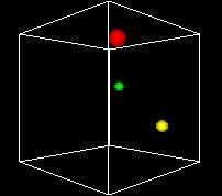
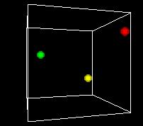
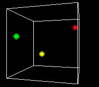
S-___. CARD: FIGURE F-3
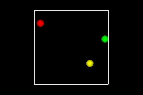 NARRATOR (CONTINUING)
Here you can see three points represented, colored red,
green and yellow just to tell them apart. So this is
a graphical display of three rows of data.
S-___. MEDIUM SHOT: NARRATOR IN FRONT OF NEUTRAL BACKGROUND
NARRATOR (CONTINUING)
If we add another column, so we have three columns of data,
now each row can be a point in 3D space...
S-___. ANIMATION A-1
NARRATOR (CONTINUING)
Here you can see three points represented, colored red,
green and yellow just to tell them apart. So this is
a graphical display of three rows of data.
S-___. MEDIUM SHOT: NARRATOR IN FRONT OF NEUTRAL BACKGROUND
NARRATOR (CONTINUING)
If we add another column, so we have three columns of data,
now each row can be a point in 3D space...
S-___. ANIMATION A-1
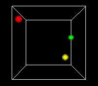
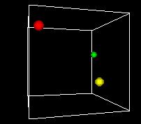
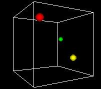
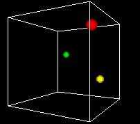
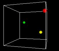
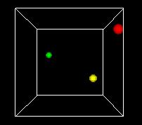
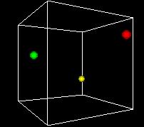
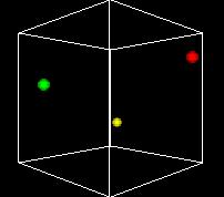
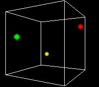
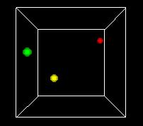 NARRATOR (CONTINUING)
This animation shows the space turning so we can get views
from different angles. One of the problems of the 3D view
is can be hard to see what's behind. Using time as an added
dimension and turning a model can help solve this problem
if we only want to see a few points in the state space.
But if we want to plot every possible point, we can't see
a whole volume of points directly, any more that we can
see inside a stack of pingpong balls..
A more fundamental problem is that -- remember -- we have up
to 22,000 dimensions in our data. We're already hitting some
problems with 3 dimensions, and we've run out. Clearly we can't
directly visualize higher-dimensional state spaces. But there
are some tricks we can do, as we'll see later.
Still another problem is that we want to be able to display
our decision function, the output of the Support Vector Machine
method. It's just a one-dimensional function, but that does
use a dimension.
So the most common approach is like the one in this figure...
S-___. CARD: FIGURE F-4
NARRATOR (CONTINUING)
This animation shows the space turning so we can get views
from different angles. One of the problems of the 3D view
is can be hard to see what's behind. Using time as an added
dimension and turning a model can help solve this problem
if we only want to see a few points in the state space.
But if we want to plot every possible point, we can't see
a whole volume of points directly, any more that we can
see inside a stack of pingpong balls..
A more fundamental problem is that -- remember -- we have up
to 22,000 dimensions in our data. We're already hitting some
problems with 3 dimensions, and we've run out. Clearly we can't
directly visualize higher-dimensional state spaces. But there
are some tricks we can do, as we'll see later.
Still another problem is that we want to be able to display
our decision function, the output of the Support Vector Machine
method. It's just a one-dimensional function, but that does
use a dimension.
So the most common approach is like the one in this figure...
S-___. CARD: FIGURE F-4
 NARRATOR (CONTINUING)
... two dimensions are used for the state space and
one is used for the decision function. Here the horizontal
dimensions represent the state space, like latitude and
longitude on a map, and the third dimension, the altitude,
is the decision function. The best choice is the lowest
in this representation, so we're looking for the bottom
of the bowl.
But there is a problem with seeing the whole state
space and decision function at once. Because paper
is flat and screens are flat, it is most common to display
a 2D state space in a 2D image, with color as the third
dimension.
S-___. FIGURE F-5
NARRATOR (CONTINUING)
... two dimensions are used for the state space and
one is used for the decision function. Here the horizontal
dimensions represent the state space, like latitude and
longitude on a map, and the third dimension, the altitude,
is the decision function. The best choice is the lowest
in this representation, so we're looking for the bottom
of the bowl.
But there is a problem with seeing the whole state
space and decision function at once. Because paper
is flat and screens are flat, it is most common to display
a 2D state space in a 2D image, with color as the third
dimension.
S-___. FIGURE F-5
         NARRATOR (CONTINUING)
      That's how the government of Australia produced this image.
      Ranges of altitudes are shown, starting at sea level, as blue,
      light blue, green, yellow, orange, red, violet and gray for
      the highest.

      This is just another way to show terrain data -- or state space data.

      [PAUSE]

S-___. MEDIUM SHOT: NARRATOR IN FRONT OF NEUTRAL BACKGROUND

         NARRATOR (CONTINUING)
      So let's see some decision function data plotted this way.

S-___. FIGURE F-6
NARRATOR (CONTINUING)
Here is a decision function for some 2D data, where
dark blue is for the lowest negative values and dark
red is for the highest positive values. The black
line is where the decision function is zero, and so the
data is "right on the line" between +, live rat or good
credit, and -, dead rat or bad credit.
S-___. MEDIUM SHOT: NARRATOR IN FRONT OF NEUTRAL BACKGROUND
NARRATOR (CONTINUING)
Remember, we're trying to show some analogies here by
boiling 22,000 dimensions of data down to 2, and then
using the third for the decision function. And I want to
emphasize that we do this not because it's a great ideas,
but because we don't know of a better way to display
these fundamental concepts. If we knew how to display
the 22,00 dimensions without boiling anything down we'd
certainly prefer it.
One thing this exercise does illustrate is the
importance of reducing dimensions if you can.
Many techniques in machine learning, including SVMs,
begin by attempting to eliminate as many dimensions
-- in other words as many columns of data -- as possible
without sacrificing quality in the decision function.
In fact, recent research by BIOwulf mathematicians
has shown that coming up with which columns to throw out
is actually more critical than coming up with an otherwise
good decision function. So we'll look at tossing out
columns first.
Assume we have some sort of workable program for creating
decision functions from training data. The most
straightforward approach would be to try every possible
subset of columns and each time, produce the decision
function using the training data and then test it using
the testing data. The find the smallest subset that
gives right answers. Simple!
Unfortunately, it's also impossible in a practical sense,
because of something called the combinatorial explosion.
S-___. CARD YELLOW LETTERS ON BLUE BACKGROUND:
combinatorial explosion
NARRATOR (CONTINUING)
To understand the combinatorial explosion, let's take a
momentary diversion into the world of subsets.
S-___. MEDIUM SHOT: NARRATOR IN FRONT OF NEUTRAL BACKGROUND
NARRATOR (CONTINUING)
First lets consider some small sets and their subsets. If you
have a set with only one thing in it, there are two possible
subsets: the original set with one thing in it and the
empty set, which you will recall is the name for a set with
nothing in it.
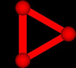
S-___. ANIMATION A-2
NARRATOR (CONTINUING)
This animation is cycling through these two options.
One thing, then nothing. Or if you prefer, nothing,
then one thing. The sphere is the one object, and
we use red to show not being in the set and green to
show being in the set. Just like red means stop and
green means go at a traffic light, here red means "no"
and green means "yes."
So far with this example it is no problem to just breeze
through all the combinations.
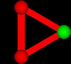
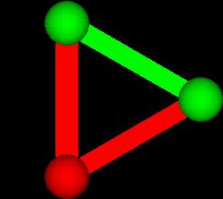
S-___. ANIMATION A-3
NARRATOR (CONTINUING)
Next consider a set of two objects. There are four subsets:
no objects, one object, the other object, or both objects.
We highlight the connection between them to emphasize that
they are in a subset together.
S-___. MEDIUM SHOT: NARRATOR IN FRONT OF NEUTRAL BACKGROUND
NARRATOR (CONTINUING)
So one object had 2 subsets, while 2 objects had 4 subsets.
What do you think, will 3 objects have 6 subsets?
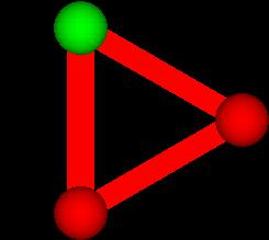
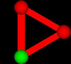
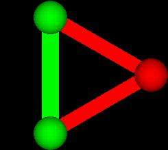
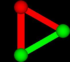
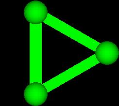
S-___. ANIMATION A-4
         NARRATOR (CONTINUING)
      As you can see in this animation, there is one way to take
      no things, three ways to take one thing, three ways to
      take two things, and one way to take three things.
      That adds up to eight subsets.

S-___. MEDIUM SHOT: NARRATOR IN FRONT OF NEUTRAL BACKGROUND

         NARRATOR (CONTINUING)
      Eight?  The sequence goes 2, 4, 8 so far.  Is it doubling
      every time? Let's see.

S-___. ANIMATION A-5
         NARRATOR (CONTINUING)
      Sure enough.  When there are four objects, there is
      one way to have no thing, four ways to have one thing,
      six ways to have two things -- four around the square
      and the two diagonals -- four ways to have three things
      and one way to have four things.

S-___. MEDIUM SHOT: NARRATOR IN FRONT OF NEUTRAL BACKGROUND

         NARRATOR (CONTINUING)
      This is getting boring.  You know why?  Because it's
      taking so long!  It is doubling every time.  That was
      sixteen subsets, and the next one, seven objects, would
      be 32 subsets.  So we're not going to do that one.  At the
      2 frames per second we've been using, it would take over
      a minute.  We promised this would be short.

      So let's jump ahead.  What if we have 30 objects?
      That's not a very big number.  A classroom of 30
      students is a common thing.  How many possible
      clubs could you form out of a classroom of thirty
      students?  If we try to count them up I don't think
      we'll make it.

S-___. ANIMATION A-6
NARRATOR (CONTINUING)
It starts out easy -- there's one way to have a club
with no students. Thirty ways to have a club with one student.
335 ways to have a club with 2 students. This is going
to take a while. Almost 3 minutes just for the clubs of two
students. While we're watching the animation run, let me talk
about how we figure this out. There's 30 ways to pick the
first student, and because they can't be in a club twice you
exclude them from the second choice, and have 29 ways to pick
the second student. But that means we've counted each club twice,
so the formula is 30 times 29 divided by 2, which is how we get 335.
As you can imagine, this is quite a pain to do for all the sizes of
clubs.
Luckily there's another way. If it doubles each time, the
general rule is that the number of subsets is just 2 to the
power of the number of objects. Call this N for number of
objects. The number of subsets is 2 raised to the N power.
2 raised to the 30th power is over a billion (that's American
billion, 1 followed by 9 zeroes). At this frame rate it will take us
17 years to watch this animation. So get comfy!
Just kidding.
[ANIMATION IS INTERRUPTED]
S-___. MEDIUM SHOT: NARRATOR IN FRONT OF NEUTRAL BACKGROUND
NARRATOR (CONTINUING)
Now you can see why we call it a combinatorial explosion.
Remember, we're dealing with data with up to 22,000 things to
correlate in subsets. Long before we get up that high
we'll be dealing with more susbsets than there are particles
in the known universe. People like to use that phrase a lot:
"more than the number of particles in the known universe."
But that's just peanuts to the combinatorial explosion. These
numbers are staggeringly bigger than that!
Allow me to quote from Douglas Adams, in The Hitchhiker's
Guide to the Galaxy.:
[HOLDS UP BOOK]
"Space is big. Really big. You just won't believe how
vastly hugely mind-bogglingly big it is. I mean, you may
think it's a long way down the road to the chemist, but
that's just peanuts to space."
Well, as you know, space is mostly devoid of matter -- the
known universe is mostly empty space. But imagine if the same
sized known universe was full of particles, as many as it could
hold. The number of subsets of 22,000 objects is mind-numbingly
bigger than the number of particles the universe could hold.
So my point, and I do have one, is that because of the
combinatorial explosion there is no way we are going
to try all possible subsets of what we are calling the
columns or the dimensions of data. So, we have to do
something else. Something smarter.
Now that we've returned from our diversion through the world
of subsets, our next concept is...
S-___. CARD YELLOW LETTERS ON BLUE BACKGROUND:
correlation
NARRATOR (CONTINUING)
...correlation. One of the most important questions
people can ask is, "why?" We want to establish causality.
The first step in that process is to establish a correlation.
S-___. CARD: FIGURE F-7
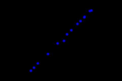 NARRATOR (CONTINUING)
In this state space plot all of the data points occur
pretty much on a line. This shows a strong correlation.
Low values of one variable always seem to be associated
with low values of the other, and high values of one
variable always seem to be associated with high values
of the other.
What we are hoping to do is to find a small number of
columns among the 22,000 that are highly correlated
with the decision function, so we can throw away the rest.
S-___. CARD YELLOW LETTERS ON BLUE BACKGROUND:
orthogonal
NARRATOR (CONTINUING)
This is related to the idea of being orthogonal.
Now don't get confused. The word orthogonal is also
used in geometry to mean at right angles. A flagpole
is orthogonal to the ground. But here it has a different,
more subtle meaning. It means roughly the opposite of
correlated. Two variables are orthogonal if they are
completely uncorrelated, if they don't affect each other
at all. This means there's no causality between them.
S-___. CARD: FIGURE F-8
NARRATOR (CONTINUING)
In this state space plot all of the data points occur
pretty much on a line. This shows a strong correlation.
Low values of one variable always seem to be associated
with low values of the other, and high values of one
variable always seem to be associated with high values
of the other.
What we are hoping to do is to find a small number of
columns among the 22,000 that are highly correlated
with the decision function, so we can throw away the rest.
S-___. CARD YELLOW LETTERS ON BLUE BACKGROUND:
orthogonal
NARRATOR (CONTINUING)
This is related to the idea of being orthogonal.
Now don't get confused. The word orthogonal is also
used in geometry to mean at right angles. A flagpole
is orthogonal to the ground. But here it has a different,
more subtle meaning. It means roughly the opposite of
correlated. Two variables are orthogonal if they are
completely uncorrelated, if they don't affect each other
at all. This means there's no causality between them.
S-___. CARD: FIGURE F-8
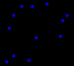 NARRATOR (CONTINUING)
If you make a state space plot -- also called a phase
plot -- of two orthogonal variables, it will look like a
random scatter. These variables were actually plotted
by rolling dice, and you can see how uncorrelated they are.
S-___. CARD YELLOW LETTERS ON BLUE BACKGROUND:
linear
NARRATOR (CONTINUING)
Our next concept is linear.
S-___. MEDIUM SHOT: NARRATOR IN FRONT OF NEUTRAL BACKGROUND
NARRATOR (CONTINUING)
This is a very important concept but it comes with a
lot of baggage. The term "non-linear" comes around
every 20 years or so and makes a big splash. It got a
lot of attention in the late 70s and early 80s with
the beginnings of chaos theory: a whole zoo of self-similar
fractals, strange attractors and chaotic bifurcations.
Unfortunately, an awful lot of people used the terms
linear and non-linear without really understanding what
they meant.
Consider this simple linear equation: y = ax - b
S-___. CARD YELLOW LETTERS ON BLUE BACKGROUND:
y = ax - b
NARRATOR (CONTINUING)
Remember that x is the variable and a and b are constants.
This is a linear equation because the most complicated term
is 'a' times 'x,' a linear relationship.
S-___. ANIMATION A-7
[Note: In this animation the narrator's finger should be
represented on a dial or knob, or else editing should be
used to incorporate live action of the narrator moving
a mouse.]
NARRATOR (CONTINUING)
The graph of this equation looks like this. You can see
that it is a straight line no matter what values 'a' and
'b' have. You may recall the idea of slop and intercept
from algebra. 'a' controls the slope of the line, and
'b' controls the Y intercept, the place where the line
intersects the vertical axis here; we show a blue sphere
at that point.
S-___. MEDIUM SHOT: NARRATOR IN FRONT OF NEUTRAL BACKGROUND
NARRATOR (CONTINUING)
This shows how a linear equation of one variable looks.
(By the way, in higher mathematics 'x' could also be a
vector or a function.)
S-___. CARD: FIGURE F-9
[THE SUM OF TWO LINEAR FUNCTIONS]
NARRATOR (CONTINUING)
If you make a state space plot -- also called a phase
plot -- of two orthogonal variables, it will look like a
random scatter. These variables were actually plotted
by rolling dice, and you can see how uncorrelated they are.
S-___. CARD YELLOW LETTERS ON BLUE BACKGROUND:
linear
NARRATOR (CONTINUING)
Our next concept is linear.
S-___. MEDIUM SHOT: NARRATOR IN FRONT OF NEUTRAL BACKGROUND
NARRATOR (CONTINUING)
This is a very important concept but it comes with a
lot of baggage. The term "non-linear" comes around
every 20 years or so and makes a big splash. It got a
lot of attention in the late 70s and early 80s with
the beginnings of chaos theory: a whole zoo of self-similar
fractals, strange attractors and chaotic bifurcations.
Unfortunately, an awful lot of people used the terms
linear and non-linear without really understanding what
they meant.
Consider this simple linear equation: y = ax - b
S-___. CARD YELLOW LETTERS ON BLUE BACKGROUND:
y = ax - b
NARRATOR (CONTINUING)
Remember that x is the variable and a and b are constants.
This is a linear equation because the most complicated term
is 'a' times 'x,' a linear relationship.
S-___. ANIMATION A-7
[Note: In this animation the narrator's finger should be
represented on a dial or knob, or else editing should be
used to incorporate live action of the narrator moving
a mouse.]
NARRATOR (CONTINUING)
The graph of this equation looks like this. You can see
that it is a straight line no matter what values 'a' and
'b' have. You may recall the idea of slop and intercept
from algebra. 'a' controls the slope of the line, and
'b' controls the Y intercept, the place where the line
intersects the vertical axis here; we show a blue sphere
at that point.
S-___. MEDIUM SHOT: NARRATOR IN FRONT OF NEUTRAL BACKGROUND
NARRATOR (CONTINUING)
This shows how a linear equation of one variable looks.
(By the way, in higher mathematics 'x' could also be a
vector or a function.)
S-___. CARD: FIGURE F-9
[THE SUM OF TWO LINEAR FUNCTIONS]
 NARRATOR (CONTINUING)
An almost magical property of linear equations is
that if you add two or more of them in any linear
combination you always get another linear equation.
Here we show visually how two linear equations are
added to produce a third.
S-___. MEDIUM SHOT: NARRATOR IN FRONT OF NEUTRAL BACKGROUND
NARRATOR (CONTINUING)
A lot of work has been done over a long period of time
coming up with techniques and tricks for solving linear
equations. At this point they represent a sort of
double-edged sword. Whenever a problem can be reduced
to a linear form it becomes much easier to analyze and
solve. But most real-world systems cannot be described
by linear equations. So we much chose between ease of
solution and accuracy.
In fact, saying linear equations are easier to solve is
a vast understatement. Consider this chart from the book
General System Theory by Ludwig von Bertalanffy, 1968.
The chapter is called "The Difficulty of Solving Equations."
S-___. TABLE T-5
NARRATOR (CONTINUING)
An almost magical property of linear equations is
that if you add two or more of them in any linear
combination you always get another linear equation.
Here we show visually how two linear equations are
added to produce a third.
S-___. MEDIUM SHOT: NARRATOR IN FRONT OF NEUTRAL BACKGROUND
NARRATOR (CONTINUING)
A lot of work has been done over a long period of time
coming up with techniques and tricks for solving linear
equations. At this point they represent a sort of
double-edged sword. Whenever a problem can be reduced
to a linear form it becomes much easier to analyze and
solve. But most real-world systems cannot be described
by linear equations. So we much chose between ease of
solution and accuracy.
In fact, saying linear equations are easier to solve is
a vast understatement. Consider this chart from the book
General System Theory by Ludwig von Bertalanffy, 1968.
The chapter is called "The Difficulty of Solving Equations."
S-___. TABLE T-5
|
Table 1.1
Classification of Mathematical Problems *
and Their Ease of Solution By Analytical Methods
After Franks, 1967
| . |
. |
. |
Linear |
. |
. |
. |
. |
Nonlinear |
. |
| Equation Type: |
One
Equation |
. |
Several
Equations |
. |
Many
Equations |
. |
One
Equation |
Several
Equations |
Many
Equations |
| Algebraic |
Trivial |
. |
Easy |
. |
Essentially Impossible |
.
| Very Difficult | Very Difficult | Impossible |
| Ordinary Differential |
Easy |
. |
Difficult |
. |
Essentially Impossible |
.
| Essentially Impossible | Impossible | Impossible |
| . |
. |
. |
x |
. |
. |
.
| . |
. |
. |
| Partial Differential |
Difficult |
. |
Essentially Impossible |
. |
Essentially Impossible |
.
| Impossible | Impossible | Impossible |
* Courtesy of Electronic Associates, Inc.
|
         NARRATOR (CONTINUING)
      Take a moment to look at this.  Down the left column are
      listed types of equations.  Of the other two columns to
      the right, one is for linear and the other for non-linear
      equations.  [PAUSE]

      Notice that all the non-linear equations are very
      difficult or worse.  Even the linear equations are pretty
      bad.  Everything to the right of the thick black line is
      pretty useless.

S-___. MEDIUM SHOT: NARRATOR IN FRONT OF NEUTRAL BACKGROUND

      Here's what the author had to say in his own dryly
      humorous style: "[these equations are], if linear,
      tiresome to solve even in the case of a few variables;
      if nonlinear, they are unsolvable except in special cases."

      So, to paraphrase an old song, we will use linear
      equations when we can and non-linear equations when we must.

S-___. CARD YELLOW LETTERS ON BLUE BACKGROUND:

   weights

         NARRATOR (CONTINUING)
      Building on the concept of linearity, our next
      concepts is weights.

S-___. MEDIUM SHOT: NARRATOR IN FRONT OF NEUTRAL BACKGROUND

         NARRATOR (CONTINUING)
      Our best hope is that we can produce a linear decision
      function, with weights for each data dimension.  We
      use the term weights to mean a set of constants, like
      'a' in the last example, only a vector of them.  We call
      this vector 'w' for weights, and it consists of a set of
      constants named w-sub-1 through w-sub-22,000 or whatever.
      So our decision function d becomes this.

S-___. CARD YELLOW LETTERS ON BLUE BACKGROUND:

   vector form

   D = w.x

   expanded

   D = w1 x1 + w2 x2 + w3 x3 +

         NARRATOR (CONTINUING)
      We use bold in the vector form to show that w and x are vectors.
      The w's and x's in the expanded form are the components of the
      vectors.

S-___. MEDIUM SHOT: NARRATOR IN FRONT OF NEUTRAL BACKGROUND

         NARRATOR (CONTINUING)
      We can visualize each x vector as a bunch of strips of cloth
      tied onto a string to become the tail of a kite.

S-___. MEDIUM SHOT: NARRATOR WITH KITE

         NARRATOR (CONTINUING)
      Didi you get that?  One vector is a kite tail, with lots of cloth strips.  Each cloth strip stands for a number.  They're called components of the vector.  One kite, one vector.  And remember, there will be lots of vectors.

      Each kite tail lands, in turn, next to the same set of weight
      values as you see in this animation...

S-___. ANIMATION A-8

   [Note: Again, in this animation the narrator's finger should be
   represented on a dial or knob, or else editing should be
   used to incorporate live action of the narrator moving
   a mouse.]


         NARRATOR (CONTINUING)
      ... each weight -- the red bars -- multiplies by its
      corresponding x -- the blue bars -- to make a weighted result
     -- the purple bars -- which are then all added together to make
     the decision function.  The only challenge is to choose the
     values of the w's correctly.

S-___. MEDIUM SHOT: NARRATOR IN FRONT OF NEUTRAL BACKGROUND

         NARRATOR (CONTINUING)
      Of course, that's the whole game.  Assuming you can live
      with a linear result, and we know how much grief that will
      save us, the decision function we just gave is the holy
      grail of machine learning.  How do you set the weights?

      From this point we'll be looking at ways that Biowulf's
      mathematicians solve this problem.  The first important tool is...

S-___. CARD YELLOW LETTERS ON BLUE BACKGROUND:

   recursion

         NARRATOR (CONTINUING)
      ... recursion.

S-___. MEDIUM SHOT: NARRATOR IN FRONT OF NEUTRAL BACKGROUND

         NARRATOR (CONTINUING)
      This is actually an idea that is actually easier
      to understand than it is to explain.

S-___. CARD: FIGURE F-10

20 MULE TEAM BORAX BOX


         NARRATOR (CONTINUING)
      There's a famous old box label for Twenty Mule Team Borax that
      shows a little girl holding a box of Twenty Mule Team Borax, and
      of course on that box is another little girl holding another box,
      and so on.

S-___. MEDIUM SHOT: NARRATOR IN FRONT OF NEUTRAL BACKGROUND

         NARRATOR (CONTINUING)
      Or perhaps this old Mad Magazine cover will help.

S-___. CARD: FIGURE F-10


         NARRATOR (CONTINUING)
      As you can see, recursion is a sort of magic trick
      that seems to create something out of nothing.  But
      it actually just involves use of the magic words
      "and so on."

      In this case, Alfred E. Neuman is holding a hat that
      contains a rabbit, and the rabbit is holding a hat that
      contains a smaller Alfred, and so on.  In this case the
      "and so on" only goes two levels down, but it's easy to
      see how it could go any number of levels, like on the
      Borax box.

S-___. MEDIUM SHOT: NARRATOR IN FRONT OF NEUTRAL BACKGROUND

         NARRATOR (CONTINUING)
      So, armed with that concept we move on to...

S-___. CARD YELLOW LETTERS ON BLUE BACKGROUND:

   recursive feature elimination

         NARRATOR (CONTINUING)
      ... recursive feature elimination.

S-___. MEDIUM SHOT: NARRATOR IN FRONT OF NEUTRAL BACKGROUND

         NARRATOR (CONTINUING)
      This is one of the methods that Biowulf's mathematicians have
      refined.  Perhaps the best way to explain it is to compare it
      to that recent hit TV show in the United States -- Survivor.
      Rather than trying to evaluate each contestant's survival
      skills alone, they tested them as a team.  This may not be
      the way to identify the best survivor, but it makes it pretty
      easy to identify the worst.

      Similarly, it is easier to analyze a set of columns of
      data in our chart to see which is least useful for deciding
      the decision function.  Then that column, or feature as it
      is called here, is eliminated and the same procedure is
      done on the remaining group, and so on. There's
      those magic words, which make it recursive feature
      elimination.

S-___. CARD YELLOW LETTERS ON BLUE BACKGROUND:

   support vectors

         NARRATOR (CONTINUING)
      Now we get to the fundamental tool used by BIOwulf's
      mathematicians: support vectors.

S-___. MEDIUM SHOT: NARRATOR IN FRONT OF NEUTRAL BACKGROUND

         NARRATOR (CONTINUING)
      And it's only fair to warn you, this is the weird part.
      What's weird about it is that it involves higher dimensions.
      Higher even than the 22,000 we mentioned before.

      But first, let me clear up some possible confusion about
      terminology.  We've been throwing a lot of specialized
      mathematical terms around here, sometimes with subtle
      distinctions.  Just like Eskimos have many words for snow,
      mathematicians have many words for dimensions.

S-___. CARD: TABLE T-6
NARRATOR (CONTINUING)
As you can see, recursion is a sort of magic trick
that seems to create something out of nothing. But
it actually just involves use of the magic words
"and so on."
In this case, Alfred E. Neuman is holding a hat that
contains a rabbit, and the rabbit is holding a hat that
contains a smaller Alfred, and so on. In this case the
"and so on" only goes two levels down, but it's easy to
see how it could go any number of levels, like on the
Borax box.
S-___. MEDIUM SHOT: NARRATOR IN FRONT OF NEUTRAL BACKGROUND
NARRATOR (CONTINUING)
So, armed with that concept we move on to...
S-___. CARD YELLOW LETTERS ON BLUE BACKGROUND:
recursive feature elimination
NARRATOR (CONTINUING)
... recursive feature elimination.
S-___. MEDIUM SHOT: NARRATOR IN FRONT OF NEUTRAL BACKGROUND
NARRATOR (CONTINUING)
This is one of the methods that Biowulf's mathematicians have
refined. Perhaps the best way to explain it is to compare it
to that recent hit TV show in the United States -- Survivor.
Rather than trying to evaluate each contestant's survival
skills alone, they tested them as a team. This may not be
the way to identify the best survivor, but it makes it pretty
easy to identify the worst.
Similarly, it is easier to analyze a set of columns of
data in our chart to see which is least useful for deciding
the decision function. Then that column, or feature as it
is called here, is eliminated and the same procedure is
done on the remaining group, and so on. There's
those magic words, which make it recursive feature
elimination.
S-___. CARD YELLOW LETTERS ON BLUE BACKGROUND:
support vectors
NARRATOR (CONTINUING)
Now we get to the fundamental tool used by BIOwulf's
mathematicians: support vectors.
S-___. MEDIUM SHOT: NARRATOR IN FRONT OF NEUTRAL BACKGROUND
NARRATOR (CONTINUING)
And it's only fair to warn you, this is the weird part.
What's weird about it is that it involves higher dimensions.
Higher even than the 22,000 we mentioned before.
But first, let me clear up some possible confusion about
terminology. We've been throwing a lot of specialized
mathematical terms around here, sometimes with subtle
distinctions. Just like Eskimos have many words for snow,
mathematicians have many words for dimensions.
S-___. CARD: TABLE T-6
| rat # | Carb. | Fat | Cholest. | Sodium | Protein | Vitamin A | Vitamin C | Calcium | Iron | +/- |
|---|
| rat #1 | 0 g | 0.5 g | 30 mg | 200 mg | 13 g | 0% | 0% | 0% | 2% | - |
| rat #2 | 20 g | 0 g | 0 mg | 10 mg | 1 g | 0% | 20% | 0% | 2% | - |
| rat #3 | 25 g | 2 g | 0 mg | 45 mg | 0 g | 0% | 0% | 0% | 2% | - |
| rat #4 | 4 g | 0 g | 0 mg | 0 mg | 1 g | 4% | 8% | 2% | 4% | + |
% = per cent daily human requirements
NARRATOR (CONTINUING)
Recall our table of which nutrients the rats were fed. We
called the rows in this table data points, points in the
state space, vectors, and sometimes test data or training
data. We called the columns in this tables variables,
dimensions and features. They're dimensions when we want
to represent them in a state space, and features when we
want to eliminate them with recursive feature elimination.
Now we're going to call them dimensions again as we do some
math tricks with them.
S-___. ANIMATION A-9
[NOTE: THIS FOOTAGE HAS ALREADY BEEN PRODUCED BY BEOWULF]
NARRATOR (CONTINUING)
Here is a 2D state space plot of some data. We'd like to
be able to find a linear function decision function that
cleanly separates the +'s from the -'s. That would
mean finding a line that separates them in this plot, but
there isn't one.
Now you can see as the animation rotates to show a third
dimension, that in a 3D state space plot there is a linear
decision function that cleanly separates the space, which
means in 3D that a plane can separate them, and you see
that one can.
S-___. MEDIUM SHOT: NARRATOR IN FRONT OF NEUTRAL BACKGROUND
NARRATOR (CONTINUING)
But what if 3 dimensions doesn't cut it? Well, we
can just add more. The problem is, as we've mentioned,
we can't show you what that looks like. The best we can do
is use some toothpicks and some miniature marshmallows
to evoke the idea.
Here I have one marshmallow. It stands for a one
dimensional point. It has -- humor me on this -- no
height, width or depth.
I move the point in some direction and trace out a line
segment. We can build that with a toothpick and another
marshmallow.
[CUT]
S-___. MEDIUM SHOT: NARRATOR IN FRONT OF NEUTRAL BACKGROUND
NARRATOR IS HOLDING MODEL OF LINE SEGMENT MADE OF
TWO MARSHMALLOWS AND A TOOTHPICK
NARRATOR (CONTINUING)
So this represents a 1-dimensional line segment which
has length, but no width or height.
If I move it at right angles the same distance, it
traces out a square. I can build that with two more
marshmallows and three more toothpicks.
[CUT]
S-___. MEDIUM SHOT: NARRATOR IN FRONT OF NEUTRAL BACKGROUND
NARRATOR IS HOLDING MODEL OF SQUARE MADE OF
FOUR MARSHMALLOWS AND FOUR TOOTHPICKS
NARRATOR (CONTINUING)
This represents a 2-dimensional square which has
length and width but no height.
If I once again move it at right angles the same
distance it traces out a cube. I can build a
cube by adding four marshmallows and eight toothpicks.
[CUT]
S-___. MEDIUM SHOT: NARRATOR IN FRONT OF NEUTRAL BACKGROUND
NARRATOR IS HOLDING MODEL OF CUBE MADE OF
EIGHT MARSHMALLOWS AND TWELVE TOOTHPICKS
NARRATOR (CONTINUING)
This represents a three-dimensional cube which has
length, width and height.
Now we'd like to do this trick again but we can't --
we've run out of dimensions. I can't even imagine what
the next step would be. There are people who claim to
be able to visualize higher dimensions, but other people
wonder if they really can.
Still, there is something we can do. We can study each
transition from one dimension to the next, and then say
what would happen by analogy.
S-___. MEDIUM SHOT: NARRATOR IN FRONT OF NEUTRAL BACKGROUND
NARRATOR (CONTINUING)
So without a visual model to guide us, we can say: "Imagine
moving the cube at right angles again, the same distance,
and tracing out a hypercube, a 4-dimensional cube.
We could build one of those with eight more marshmallows and
20 more toothpicks."
Now, I have no idea what that means, and we don't have that
extra fourth dimension to try it in. But the point is, a
lot can be figured out by analogy. We know how the math
works at any dimension, up to infinite dimensions, believe
it or not. And luckily, we don't need to visualize the
problem to solve it -- only to explain it! That's why we're
better at solving it than explaining it.
Okay, I've been jollying you along here with this higher
dimension stuff to prepare you for this next statement.
It probably won't make perfect sense, but it's the best
we can do.
The Support Vector Machine -- SVM -- method, works this way.
It keeps adding dimensions until it can find a hyperplane to
split the state space, which means there is a linear decision
function. Then it finds all the data vectors that are closest
to this hyper-plane. These are called the support vectors.
Then the support vectors are used to do recursive feature
elimination and to create the decision function.
Let me run through that again.
The SVM method keeps adding dimensions until it can
find a hyper-plane -- a higher-dimensional plane -- to split
the state space, which means there is a linear decision function.
Then it finds all the data vectors that are closest to this
hyper-plane. These are called the support vectors. Then the
support vectors are used to do recursive feature elimination
and to create the decision function.
Now one thing that's interesting about this is that we
started out wanting to throw away columns, and we did,
but we also threw away rows! Any vectors which are not
support vectors are thrown away and not used for the
calculating the decision function.
Okay, I know your mind is swirling. Maybe some pictures
will help.
S-___. CARD: FIGURE F-11
 NARRATOR (CONTINUING)
The following images are taken from an interactive Java
Applet written by Hong Zhang of BIOwulf.
Now once again we have the advantages and disadvantages
of being back in 2 dimensions. It's good because we can
see the whole state space at once, but it's bad because
it can't show any of the higher dimensional data.
The way this Applet works is the user places data points in a
white rectangle, black dots for the pluses and open dots for
the minuses. Then the Applet chooses the support vectors
and computes the decision function using the SVM method.
Next the decision function is displayed as color, red
being the low negative values and blue the high positive
values. The data points chosen to be support vectors are
circled.
S-___. MEDIUM SHOT: NARRATOR IN FRONT OF NEUTRAL BACKGROUND
NARRATOR (CONTINUING)
This was for a linear decision function. Here's how it
looks if we allow a non-linear decision function.
S-___. CARD: FIGURE F-12
NARRATOR (CONTINUING)
The following images are taken from an interactive Java
Applet written by Hong Zhang of BIOwulf.
Now once again we have the advantages and disadvantages
of being back in 2 dimensions. It's good because we can
see the whole state space at once, but it's bad because
it can't show any of the higher dimensional data.
The way this Applet works is the user places data points in a
white rectangle, black dots for the pluses and open dots for
the minuses. Then the Applet chooses the support vectors
and computes the decision function using the SVM method.
Next the decision function is displayed as color, red
being the low negative values and blue the high positive
values. The data points chosen to be support vectors are
circled.
S-___. MEDIUM SHOT: NARRATOR IN FRONT OF NEUTRAL BACKGROUND
NARRATOR (CONTINUING)
This was for a linear decision function. Here's how it
looks if we allow a non-linear decision function.
S-___. CARD: FIGURE F-12
 NARRATOR (CONTINUING)
You can see that the data won't permit a line to divide
the state space, so a curve is needed. In this cave the
curve is defined by a third order polynomial. This is an
equation with no more complex terms than x cubed.
S-___. MEDIUM SHOT: NARRATOR IN FRONT OF NEUTRAL BACKGROUND
NARRATOR (CONTINUING)
Let's take a look at an animated sequence of these.
S-___. CARD: FIGURE F-13 (f01.gif)
NARRATOR (CONTINUING)
You can see that the data won't permit a line to divide
the state space, so a curve is needed. In this cave the
curve is defined by a third order polynomial. This is an
equation with no more complex terms than x cubed.
S-___. MEDIUM SHOT: NARRATOR IN FRONT OF NEUTRAL BACKGROUND
NARRATOR (CONTINUING)
Let's take a look at an animated sequence of these.
S-___. CARD: FIGURE F-13 (f01.gif)
 NARRATOR (CONTINUING)
We started out with a grid of nine data points. The three
upper rightmost were minuses while the rest were pluses.
Three points near the dividing line were chosen by the
Applet to be support vectors, and the decision function
follows a slight curve down the middle, though it bends
more elsewhere.
Next we added another "plus" data point, near the center,
just up and to the right of the center point. We let the
Applet compute again, and...
S-___. CARD: FIGURE F-14 (f02.gif)
NARRATOR (CONTINUING)
We started out with a grid of nine data points. The three
upper rightmost were minuses while the rest were pluses.
Three points near the dividing line were chosen by the
Applet to be support vectors, and the decision function
follows a slight curve down the middle, though it bends
more elsewhere.
Next we added another "plus" data point, near the center,
just up and to the right of the center point. We let the
Applet compute again, and...
S-___. CARD: FIGURE F-14 (f02.gif)
 NARRATOR (CONTINUING)
... now you can see the Applet has chosen the new point to
replace the center point as a support vector, and moved the
decision function a little, but there are still only three
support vectors.
S-___. CARD: FIGURE F-15 (f03.gif)
NARRATOR (CONTINUING)
... now you can see the Applet has chosen the new point to
replace the center point as a support vector, and moved the
decision function a little, but there are still only three
support vectors.
S-___. CARD: FIGURE F-15 (f03.gif)
 NARRATOR (CONTINUING)
Now we add a few more data points, this time minuses,
farther to the upper right of the center. We let the
Applet compute once again ...
S-___. CARD: FIGURE F-16 (f04.gif)
NARRATOR (CONTINUING)
Now we add a few more data points, this time minuses,
farther to the upper right of the center. We let the
Applet compute once again ...
S-___. CARD: FIGURE F-16 (f04.gif)
 NARRATOR (CONTINUING)
... and now you can see the Applet has added one of the new
points as a support vector, and dropped the one in the upper
left, but still has only three of them. Of course it has
moved the decision function again.
S-___. CARD: FIGURE F-17 (f05.gif)
NARRATOR (CONTINUING)
... and now you can see the Applet has added one of the new
points as a support vector, and dropped the one in the upper
left, but still has only three of them. Of course it has
moved the decision function again.
S-___. CARD: FIGURE F-17 (f05.gif)
 NARRATOR (CONTINUING)
Here's another positive data point added...
S-___. CARD: FIGURE F-18 (f06.gif)
NARRATOR (CONTINUING)
Here's another positive data point added...
S-___. CARD: FIGURE F-18 (f06.gif)
 NARRATOR (CONTINUING)
... and it gets chosen to be a support vector. The decision
function nows jumps more dramatically.
S-___. CARD: FIGURE F-19 (f07.gif)
NARRATOR (CONTINUING)
... and it gets chosen to be a support vector. The decision
function nows jumps more dramatically.
S-___. CARD: FIGURE F-19 (f07.gif)
 NARRATOR (CONTINUING)
Here's another positive data point added...
S-___. CARD: FIGURE F-20 (f08.gif)
NARRATOR (CONTINUING)
Here's another positive data point added...
S-___. CARD: FIGURE F-20 (f08.gif)
 NARRATOR (CONTINUING)
... and it gets chosen to be a support vector. The decision
function is tightening up as we give it finer and finer distinctions.
S-___. CARD: FIGURE F-21 (f09.gif)
NARRATOR (CONTINUING)
... and it gets chosen to be a support vector. The decision
function is tightening up as we give it finer and finer distinctions.
S-___. CARD: FIGURE F-21 (f09.gif)
 NARRATOR (CONTINUING)
Now we've hopped down to region lower and right of center,
and put another negative data point near the dividing line.
S-___. CARD: FIGURE F-22 (f10.gif)
NARRATOR (CONTINUING)
Now we've hopped down to region lower and right of center,
and put another negative data point near the dividing line.
S-___. CARD: FIGURE F-22 (f10.gif)
 NARRATOR (CONTINUING)
... and it gets chosen to be a support vector. But note that
now there are four circled points -- four support vectors.
The support vector machine needs more data points to define
the decision function.
S-___. CARD: FIGURE F-23 (f11.gif)
NARRATOR (CONTINUING)
... and it gets chosen to be a support vector. But note that
now there are four circled points -- four support vectors.
The support vector machine needs more data points to define
the decision function.
S-___. CARD: FIGURE F-23 (f11.gif)
 NARRATOR (CONTINUING)
Here's another negative data point added, advancing into
what was clearly positive territory.
S-___. CARD: FIGURE F-24 (f12.gif)
NARRATOR (CONTINUING)
Here's another negative data point added, advancing into
what was clearly positive territory.
S-___. CARD: FIGURE F-24 (f12.gif)
 NARRATOR (CONTINUING)
... and it gets chosen to be a support vector, replacing the
previous point. But notice that the positive data point in
the lower right has also bbeen made a support vector, totaling
five. The decision function is really tightening up now.
S-___. CARD: FIGURE F-25 (f13.gif)
NARRATOR (CONTINUING)
... and it gets chosen to be a support vector, replacing the
previous point. But notice that the positive data point in
the lower right has also bbeen made a support vector, totaling
five. The decision function is really tightening up now.
S-___. CARD: FIGURE F-25 (f13.gif)
 NARRATOR (CONTINUING)
Once again we add another negative data point in what was
previously positive territory.
S-___. CARD: FIGURE F-26 (f14.gif)
NARRATOR (CONTINUING)
Woah! The decision function just got wider and more curved!
And the number of support vectors has increased again --
now there are six. Each I time I add a point in the wrong
territory I'm violating its assumptions, so it has to make
a subtler decision function.
S-___. CARD: FIGURE F-27 (f15.gif)
NARRATOR (CONTINUING)
Once again we add another negative data point in what was
previously positive territory.
S-___. CARD: FIGURE F-26 (f14.gif)
NARRATOR (CONTINUING)
Woah! The decision function just got wider and more curved!
And the number of support vectors has increased again --
now there are six. Each I time I add a point in the wrong
territory I'm violating its assumptions, so it has to make
a subtler decision function.
S-___. CARD: FIGURE F-27 (f15.gif)
 NARRATOR (CONTINUING)
Okay, we add one last negative data point the same way.
S-___. CARD: FIGURE F-28 (f16.gif)
NARRATOR (CONTINUING)
Okay, we add one last negative data point the same way.
S-___. CARD: FIGURE F-28 (f16.gif)
 NARRATOR (CONTINUING)
... and it gets chosen to be a support vector, along with
another point -- now there are eight!. The decision
function has twisted and widened to accommodate the more
stringent data.
S-___. MEDIUM SHOT: NARRATOR IN FRONT OF NEUTRAL BACKGROUND
NARRATOR (CONTINUING)
Well, we could go on like this all day. It is fascinating
to watch, and even more fascinating to interact with the
Applet yourself.
But now lets look at something you don't see when you
play with the Applet. The following animation shows
those frames we just went through speeded up, with the
compute time removed.
S-___. ANIMATION A-10
NARRATOR (CONTINUING)
... and it gets chosen to be a support vector, along with
another point -- now there are eight!. The decision
function has twisted and widened to accommodate the more
stringent data.
S-___. MEDIUM SHOT: NARRATOR IN FRONT OF NEUTRAL BACKGROUND
NARRATOR (CONTINUING)
Well, we could go on like this all day. It is fascinating
to watch, and even more fascinating to interact with the
Applet yourself.
But now lets look at something you don't see when you
play with the Applet. The following animation shows
those frames we just went through speeded up, with the
compute time removed.
S-___. ANIMATION A-10
 NARRATOR (CONTINUING)
It's a thing of beauty. Sometimes the eye can pick out
patterns in motion that we don't see any other way.
Well, enough of that.
S-___. MEDIUM SHOT: NARRATOR IN FRONT OF NEUTRAL BACKGROUND
NARRATOR (CONTINUING)
I hope this is giving you a sense of what the Support
Vector Machine method does. Unfortunately, we can show
you 2 dimensions but all the real benefits occur with
much higher dimensions, which we can't show you.
S-___. CARD YELLOW LETTERS ON BLUE BACKGROUND:
kernels
NARRATOR (CONTINUING)
Kernels.
S-___. MEDIUM SHOT: NARRATOR IN FRONT OF NEUTRAL BACKGROUND
NARRATOR (CONTINUING)
This is the last concept. Is your brain full yet?
We told you earlier how a Support Vector Machine is looking
for correlations. Well, the way a SVM measures correlations
is with a function, called K, the Kernel function,
which the user must provide. It turns out there's more than
one good way to measure correlation, it depends on the data.
Some data worls better with one, other data with another.
This is one reason why mathematical experts like BIOwulf's
are still needed, and the whole process can't be autoimated, yet.
For any given type of data, like rat diets or a particular
tissue sample, there is an optimum kernel, which an experienced
mathematician can determine.
Well, I'm sure some of this made perfect sense, and
some of it seemed like mumbo jumbo. It's that way to
most of us, too. But the proof, they say, is in the pudding.
Now that we've done a survey of the mathematical tools
used by BIOwulf, let's ask the most important question:
S-___. CARD YELLOW LETTERS ON BLUE BACKGROUND:
Does it work?
NARRATOR (CONTINUING)
Does it work?
S-___. MEDIUM SHOT: NARRATOR IN FRONT OF NEUTRAL BACKGROUND
NARRATOR (CONTINUING)
Well, the short answer to this is: it sure does!
In the paper "Gene Selection for Colon Classification
using Support Vector Machines by Isabelle Guyon, Jason
Weston, Stephen Barnhill, and Vladimir Vapnik, the story
is told of these 62 biopsies samples we mentioned earlier.
They report that SVM is better than the next best known
technique with 95.8% confidence. Furthermore, the SVM
used 8 instead of 32 genes to make the classification,
after recursive feature elimination, and still had a
lower error rate.
Remember that this was from frozen tissue samples that
were combined with 30 years of follow-up patient data.
This stuff can save lives!
It was also interesting to find that other methods
falsely associated the presence of skin cell genes
with cancerous cells, just because cancerous tissue
samples tended to have more skin cells while healthy
samples had more muscle cells. The SVM method did not
make this false correlation. Also, the SVM method
did correlate lack cancer with the presence
of genes from a tiny parasite, a protozoa named
Trypanosoma, indigenous to Africa and South America.
To quote the paper: "We thought this may be an anomaly
of our gene selection method or an error in the data,
until we discovered that clinical studies report that
patients infected by Trypanosoma -- a colon parasite
-- develop resistance against colon cancer."
Clearly we need to put this new tool to work on medical diagnosis
right away!
Thank you for your time in viewing this explanatory video.
For more information about BIOwulf, see our website at
www.biowulf.com.
S-___. SCROLLING TITLES: CREDITS
DOWNWARD SCROLLING YELLOW LETTERS ON WATERFALL BACKGROUND:
Written, Directed and Edited by Alan Scrivener.
Narrated by Mollie Tobin.
Computer graphics by Alan Scrivener.
Geographical visualizations by Jeff Sale.
Special thanks to Wayne Holder and Bob Zawalnicki.
Produced by Human Interface Prototypes
for Mindtel Corp.
Filmed at the San Diego Public Library,
Mission San Diego de Alcala,
and Mission Trails Regional Park,
San Diego, California.
(C) 2001 Mindtel Corp.
Keep wondering.
NARRATOR (CONTINUING)
It's a thing of beauty. Sometimes the eye can pick out
patterns in motion that we don't see any other way.
Well, enough of that.
S-___. MEDIUM SHOT: NARRATOR IN FRONT OF NEUTRAL BACKGROUND
NARRATOR (CONTINUING)
I hope this is giving you a sense of what the Support
Vector Machine method does. Unfortunately, we can show
you 2 dimensions but all the real benefits occur with
much higher dimensions, which we can't show you.
S-___. CARD YELLOW LETTERS ON BLUE BACKGROUND:
kernels
NARRATOR (CONTINUING)
Kernels.
S-___. MEDIUM SHOT: NARRATOR IN FRONT OF NEUTRAL BACKGROUND
NARRATOR (CONTINUING)
This is the last concept. Is your brain full yet?
We told you earlier how a Support Vector Machine is looking
for correlations. Well, the way a SVM measures correlations
is with a function, called K, the Kernel function,
which the user must provide. It turns out there's more than
one good way to measure correlation, it depends on the data.
Some data worls better with one, other data with another.
This is one reason why mathematical experts like BIOwulf's
are still needed, and the whole process can't be autoimated, yet.
For any given type of data, like rat diets or a particular
tissue sample, there is an optimum kernel, which an experienced
mathematician can determine.
Well, I'm sure some of this made perfect sense, and
some of it seemed like mumbo jumbo. It's that way to
most of us, too. But the proof, they say, is in the pudding.
Now that we've done a survey of the mathematical tools
used by BIOwulf, let's ask the most important question:
S-___. CARD YELLOW LETTERS ON BLUE BACKGROUND:
Does it work?
NARRATOR (CONTINUING)
Does it work?
S-___. MEDIUM SHOT: NARRATOR IN FRONT OF NEUTRAL BACKGROUND
NARRATOR (CONTINUING)
Well, the short answer to this is: it sure does!
In the paper "Gene Selection for Colon Classification
using Support Vector Machines by Isabelle Guyon, Jason
Weston, Stephen Barnhill, and Vladimir Vapnik, the story
is told of these 62 biopsies samples we mentioned earlier.
They report that SVM is better than the next best known
technique with 95.8% confidence. Furthermore, the SVM
used 8 instead of 32 genes to make the classification,
after recursive feature elimination, and still had a
lower error rate.
Remember that this was from frozen tissue samples that
were combined with 30 years of follow-up patient data.
This stuff can save lives!
It was also interesting to find that other methods
falsely associated the presence of skin cell genes
with cancerous cells, just because cancerous tissue
samples tended to have more skin cells while healthy
samples had more muscle cells. The SVM method did not
make this false correlation. Also, the SVM method
did correlate lack cancer with the presence
of genes from a tiny parasite, a protozoa named
Trypanosoma, indigenous to Africa and South America.
To quote the paper: "We thought this may be an anomaly
of our gene selection method or an error in the data,
until we discovered that clinical studies report that
patients infected by Trypanosoma -- a colon parasite
-- develop resistance against colon cancer."
Clearly we need to put this new tool to work on medical diagnosis
right away!
Thank you for your time in viewing this explanatory video.
For more information about BIOwulf, see our website at
www.biowulf.com.
S-___. SCROLLING TITLES: CREDITS
DOWNWARD SCROLLING YELLOW LETTERS ON WATERFALL BACKGROUND:
Written, Directed and Edited by Alan Scrivener.
Narrated by Mollie Tobin.
Computer graphics by Alan Scrivener.
Geographical visualizations by Jeff Sale.
Special thanks to Wayne Holder and Bob Zawalnicki.
Produced by Human Interface Prototypes
for Mindtel Corp.
Filmed at the San Diego Public Library,
Mission San Diego de Alcala,
and Mission Trails Regional Park,
San Diego, California.
(C) 2001 Mindtel Corp.
Keep wondering.
Last update 19-Jul-2001 11:59 PM PDT by ABS.